23.1. Using Jupyter Notebooks¶ Open the notebook in SageMaker Studio Lab
This section describes how to edit and run the code in each section of this book using the Jupyter Notebook. Make sure you have installed Jupyter and downloaded the code as described in Installation. If you want to know more about Jupyter see the excellent tutorial in their documentation.
23.1.1. Editing and Running the Code Locally
Suppose that the local path of the book’s code is xx/yy/d2l-en/. Use
the shell to change the directory to this path (cd xx/yy/d2l-en) and
run the command jupyter notebook. If your browser does not do this
automatically, open http://localhost:8888 and you will see the interface
of Jupyter and all the folders containing the code of the book, as shown
in Fig. 23.1.1.
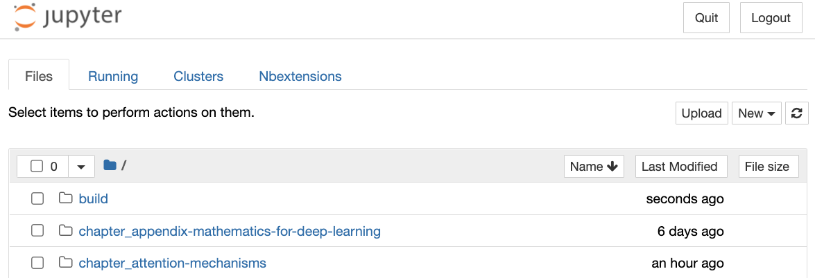
Fig. 23.1.1 The folders containing the code of this book.
You can access the notebook files by clicking on the folder displayed on the webpage. They usually have the suffix “.ipynb”. For the sake of brevity, we create a temporary “test.ipynb” file. The content displayed after you click it is shown in Fig. 23.1.2. This notebook includes a markdown cell and a code cell. The content in the markdown cell includes “This Is a Title” and “This is text.”. The code cell contains two lines of Python code.
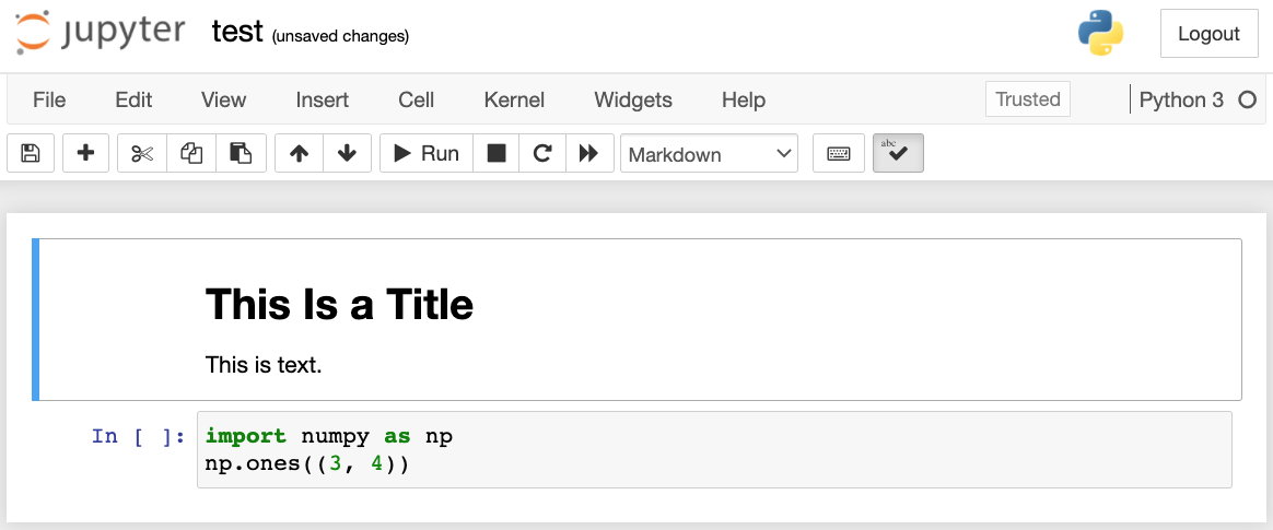
Fig. 23.1.2 Markdown and code cells in the “text.ipynb” file.
Double click on the markdown cell to enter edit mode. Add a new text string “Hello world.” at the end of the cell, as shown in Fig. 23.1.3.
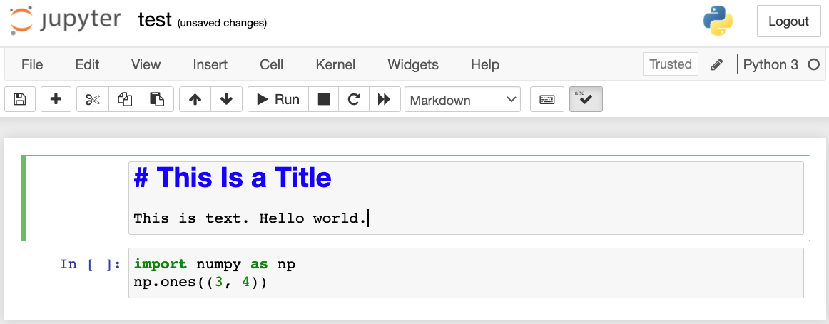
Fig. 23.1.3 Edit the markdown cell.
As demonstrated in Fig. 23.1.4, click “Cell” \(\rightarrow\) “Run Cells” in the menu bar to run the edited cell.
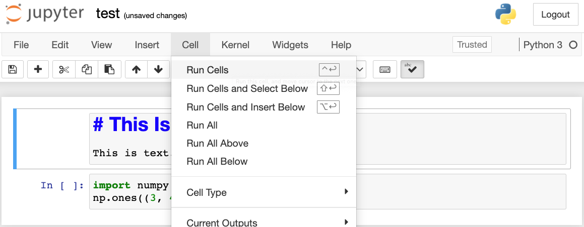
Fig. 23.1.4 Run the cell.
After running, the markdown cell is shown in Fig. 23.1.5.
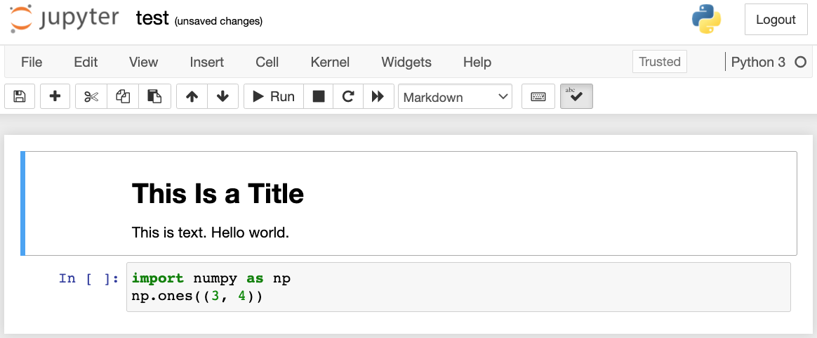
Fig. 23.1.5 The markdown cell after running.
Next, click on the code cell. Multiply the elements by 2 after the last line of code, as shown in Fig. 23.1.6.
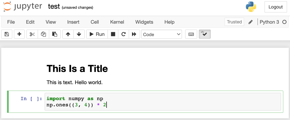
Fig. 23.1.6 Edit the code cell.
You can also run the cell with a shortcut (“Ctrl + Enter” by default) and obtain the output result from Fig. 23.1.7.
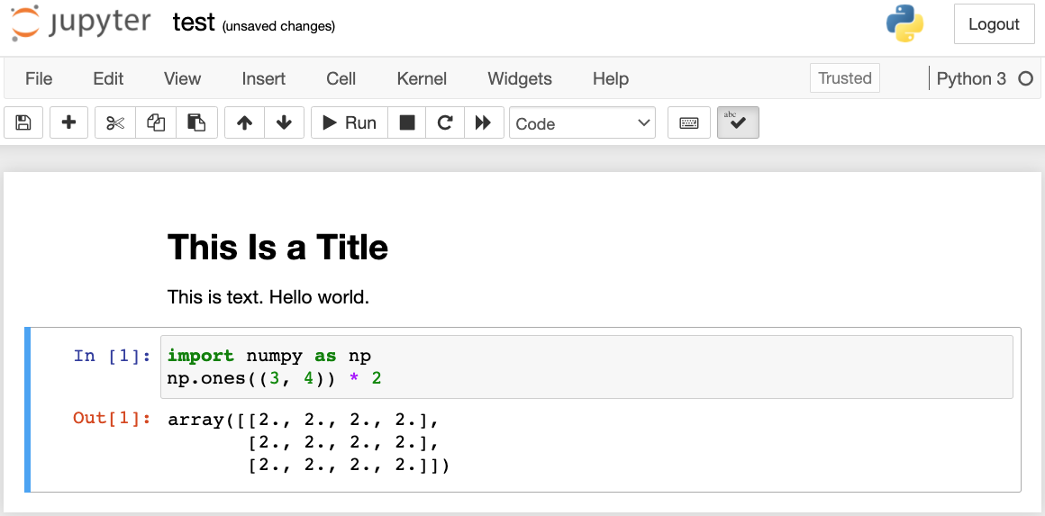
Fig. 23.1.7 Run the code cell to obtain the output.
When a notebook contains more cells, we can click “Kernel” \(\rightarrow\) “Restart & Run All” in the menu bar to run all the cells in the entire notebook. By clicking “Help” \(\rightarrow\) “Edit Keyboard Shortcuts” in the menu bar, you can edit the shortcuts according to your preferences.
23.1.2. Advanced Options
Beyond local editing two things are quite important: editing the notebooks in the markdown format and running Jupyter remotely. The latter matters when we want to run the code on a faster server. The former matters since Jupyter’s native ipynb format stores a lot of auxiliary data that is irrelevant to the content, mostly related to how and where the code is run. This is confusing for Git, making reviewing contributions very difficult. Fortunately there is an alternative—native editing in the markdown format.
23.1.2.1. Markdown Files in Jupyter
If you wish to contribute to the content of this book, you need to modify the source file (md file, not ipynb file) on GitHub. Using the notedown plugin we can modify notebooks in the md format directly in Jupyter.
First, install the notedown plugin, run the Jupyter Notebook, and load the plugin:
pip install d2l-notedown  # You may need to uninstall the original notedown.
jupyter notebook --NotebookApp.contents_manager_class='notedown.NotedownContentsManager'
You may also turn on the notedown plugin by default whenever you run the Jupyter Notebook. First, generate a Jupyter Notebook configuration file (if it has already been generated, you can skip this step).
jupyter notebook --generate-config
Then, add the following line to the end of the Jupyter Notebook
configuration file (for Linux or macOS, usually in the path
~/.jupyter/jupyter_notebook_config.py):
c.NotebookApp.contents_manager_class = 'notedown.NotedownContentsManager'
After that, you only need to run the jupyter notebook command to
turn on the notedown plugin by default.
23.1.2.2. Running Jupyter Notebooks on a Remote Server
Sometimes, you may want to run Jupyter notebooks on a remote server and access it through a browser on your local computer. If Linux or macOS is installed on your local machine (Windows can also support this function through third-party software such as PuTTY), you can use port forwarding:
ssh myserver -L 8888:localhost:8888
The above string myserver is the address of the remote server. Then
we can use http://localhost:8888 to access the remote server
myserver that runs Jupyter notebooks. We will detail on how to run
Jupyter notebooks on AWS instances later in this appendix.
23.1.2.3. Timing
We can use the ExecuteTime plugin to time the execution of each code
cell in Jupyter notebooks. Use the following commands to install the
plugin:
pip install jupyter_contrib_nbextensions
jupyter contrib nbextension install --user
jupyter nbextension enable execute_time/ExecuteTime
23.1.3. Summary
Using the Jupyter Notebook tool, we can edit, run, and contribute to each section of the book.
We can run Jupyter notebooks on remote servers using port forwarding.
23.1.4. Exercises
Edit and run the code in this book with the Jupyter Notebook on your local machine.
Edit and run the code in this book with the Jupyter Notebook remotely via port forwarding.
Compare the running time of the operations \(\mathbf{A}^\top \mathbf{B}\) and \(\mathbf{A} \mathbf{B}\) for two square matrices in \(\mathbb{R}^{1024 \times 1024}\). Which one is faster?