5.7. Predicting House Prices on Kaggle¶ Open the notebook in SageMaker Studio Lab
Now that we have introduced some basic tools for building and training deep networks and regularizing them with techniques including weight decay and dropout, we are ready to put all this knowledge into practice by participating in a Kaggle competition. The house price prediction competition is a great place to start. The data is fairly generic and do not exhibit exotic structure that might require specialized models (as audio or video might). This dataset, collected by De Cock (2011), covers house prices in Ames, Iowa from the period 2006–2010. It is considerably larger than the famous Boston housing dataset of Harrison and Rubinfeld (1978), boasting both more examples and more features.
In this section, we will walk you through details of data preprocessing, model design, and hyperparameter selection. We hope that through a hands-on approach, you will gain some intuitions that will guide you in your career as a data scientist.
%matplotlib inline
import pandas as pd
import torch
from torch import nn
from d2l import torch as d2l
%matplotlib inline
import pandas as pd
from mxnet import autograd, gluon, init, np, npx
from mxnet.gluon import nn
from d2l import mxnet as d2l

npx.set_np()
%matplotlib inline
import jax
import numpy as np
import pandas as pd
from jax import numpy as jnp
from d2l import jax as d2l
No GPU/TPU found, falling back to CPU. (Set TF_CPP_MIN_LOG_LEVEL=0 and rerun for more info.)
%matplotlib inline
import pandas as pd
import tensorflow as tf
from d2l import tensorflow as d2l
5.7.1. Downloading Data
Throughout the book, we will train and test models on various downloaded datasets. Here, we implement two utility functions for downloading and extracting zip or tar files. Again, we skip implementation details of such utility functions.
def download(url, folder, sha1_hash=None):
    """Download a file to folder and return the local filepath."""

def extract(filename, folder):
    """Extract a zip/tar file into folder."""
5.7.2. Kaggle
Kaggle is a popular platform that hosts machine learning competitions. Each competition centers on a dataset and many are sponsored by stakeholders who offer prizes to the winning solutions. The platform helps users to interact via forums and shared code, fostering both collaboration and competition. While leaderboard chasing often spirals out of control, with researchers focusing myopically on preprocessing steps rather than asking fundamental questions, there is also tremendous value in the objectivity of a platform that facilitates direct quantitative comparisons among competing approaches as well as code sharing so that everyone can learn what did and did not work. If you want to participate in a Kaggle competition, you will first need to register for an account (see Fig. 5.7.1).

Fig. 5.7.1 The Kaggle website.
On the house price prediction competition page, as illustrated in Fig. 5.7.2, you can find the dataset (under the “Data” tab), submit predictions, and see your ranking, The URL is right here:
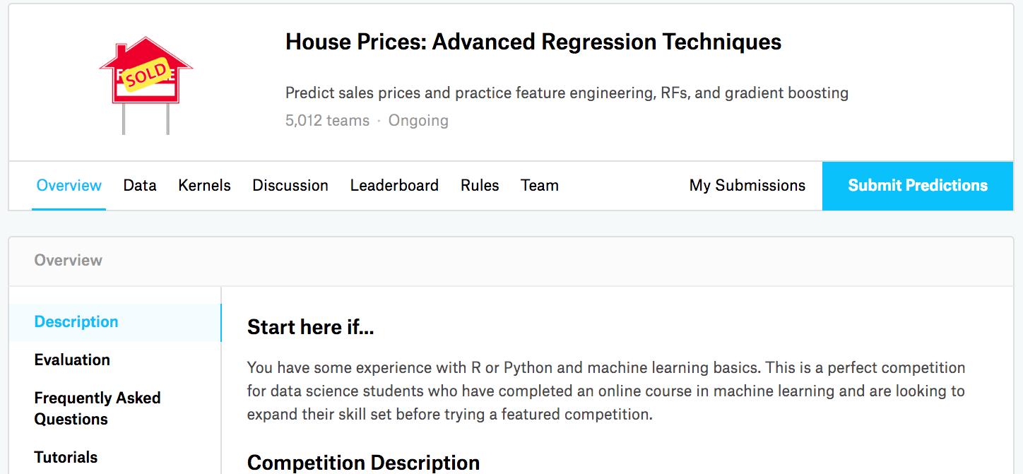
Fig. 5.7.2 The house price prediction competition page.
5.7.3. Accessing and Reading the Dataset
Note that the competition data is separated into training and test sets. Each record includes the property value of the house and attributes such as street type, year of construction, roof type, basement condition, etc. The features consist of various data types. For example, the year of construction is represented by an integer, the roof type by discrete categorical assignments, and other features by floating point numbers. And here is where reality complicates things: for some examples, some data is altogether missing with the missing value marked simply as “na”. The price of each house is included for the training set only (it is a competition after all). We will want to partition the training set to create a validation set, but we only get to evaluate our models on the official test set after uploading predictions to Kaggle. The “Data” tab on the competition tab in Fig. 5.7.2 has links for downloading the data.
To get started, we will read in and process the data using pandas,
which we introduced in Section 2.2. For convenience, we can
download and cache the Kaggle housing dataset. If a file corresponding
to this dataset already exists in the cache directory and its SHA-1
matches sha1_hash, our code will use the cached file to avoid
clogging up your Internet with redundant downloads.
class KaggleHouse(d2l.DataModule):
    def __init__(self, batch_size, train=None, val=None):
        super().__init__()
        self.save_hyperparameters()
        if self.train is None:
            self.raw_train = pd.read_csv(d2l.download(
                d2l.DATA_URL + 'kaggle_house_pred_train.csv', self.root,
                sha1_hash='585e9cc93e70b39160e7921475f9bcd7d31219ce'))
            self.raw_val = pd.read_csv(d2l.download(
                d2l.DATA_URL + 'kaggle_house_pred_test.csv', self.root,
                sha1_hash='fa19780a7b011d9b009e8bff8e99922a8ee2eb90'))
The training dataset includes 1460 examples, 80 features, and one label, while the validation data contains 1459 examples and 80 features.
data = KaggleHouse(batch_size=64)
print(data.raw_train.shape)
print(data.raw_val.shape)
Downloading ../data/kaggle_house_pred_train.csv from http://d2l-data.s3-accelerate.amazonaws.com/kaggle_house_pred_train.csv...
Downloading ../data/kaggle_house_pred_test.csv from http://d2l-data.s3-accelerate.amazonaws.com/kaggle_house_pred_test.csv...
(1460, 81)
(1459, 80)
5.7.4. Data Preprocessing
Let’s take a look at the first four and final two features as well as the label (SalePrice) from the first four examples.
print(data.raw_train.iloc[:4, [0, 1, 2, 3, -3, -2, -1]])
   Id  MSSubClass MSZoning  LotFrontage SaleType SaleCondition  SalePrice
0   1          60       RL         65.0       WD        Normal     208500
1   2          20       RL         80.0       WD        Normal     181500
2   3          60       RL         68.0       WD        Normal     223500
3   4          70       RL         60.0       WD       Abnorml     140000
We can see that in each example, the first feature is the identifier. This helps the model determine each training example. While this is convenient, it does not carry any information for prediction purposes. Hence, we will remove it from the dataset before feeding the data into the model. Furthermore, given a wide variety of data types, we will need to preprocess the data before we can start modeling.
Let’s start with the numerical features. First, we apply a heuristic, replacing all missing values by the corresponding feature’s mean. Then, to put all features on a common scale, we standardize the data by rescaling features to zero mean and unit variance:
where \(\mu\) and \(\sigma\) denote mean and standard deviation, respectively. To verify that this indeed transforms our feature (variable) such that it has zero mean and unit variance, note that \(E[\frac{x-\mu}{\sigma}] = \frac{\mu - \mu}{\sigma} = 0\) and that \(E[(x-\mu)^2] = (\sigma^2 + \mu^2) - 2\mu^2+\mu^2 = \sigma^2\). Intuitively, we standardize the data for two reasons. First, it proves convenient for optimization. Second, because we do not know a priori which features will be relevant, we do not want to penalize coefficients assigned to one feature more than any other.
Next we deal with discrete values. These include features such as
“MSZoning”. We replace them by a one-hot encoding in the same way that
we earlier transformed multiclass labels into vectors (see
Section 4.1.1). For instance, “MSZoning”
assumes the values “RL” and “RM”. Dropping the “MSZoning” feature, two
new indicator features “MSZoning_RL” and “MSZoning_RM” are created with
values being either 0 or 1. According to one-hot encoding, if the
original value of “MSZoning” is “RL”, then “MSZoning_RL” is 1 and
“MSZoning_RM” is 0. The pandas package does this automatically for
us.
@d2l.add_to_class(KaggleHouse)
def preprocess(self):
    # Remove the ID and label columns
    label = 'SalePrice'
    features = pd.concat(
        (self.raw_train.drop(columns=['Id', label]),
         self.raw_val.drop(columns=['Id'])))
    # Standardize numerical columns
    numeric_features = features.dtypes[features.dtypes!='object'].index
    features[numeric_features] = features[numeric_features].apply(
        lambda x: (x - x.mean()) / (x.std()))
    # Replace NAN numerical features by 0
    features[numeric_features] = features[numeric_features].fillna(0)
    # Replace discrete features by one-hot encoding
    features = pd.get_dummies(features, dummy_na=True)
    # Save preprocessed features
    self.train = features[:self.raw_train.shape[0]].copy()
    self.train[label] = self.raw_train[label]
    self.val = features[self.raw_train.shape[0]:].copy()
You can see that this conversion increases the number of features from 79 to 331 (excluding ID and label columns).
data.preprocess()
data.train.shape
(1460, 331)
data.preprocess()
data.train.shape
(1460, 331)
data.preprocess()
data.train.shape
(1460, 331)
data.preprocess()
data.train.shape
(1460, 331)
5.7.5. Error Measure
To get started we will train a linear model with squared loss. Not surprisingly, our linear model will not lead to a competition-winning submission but it does provide a sanity check to see whether there is meaningful information in the data. If we cannot do better than random guessing here, then there might be a good chance that we have a data processing bug. And if things work, the linear model will serve as a baseline giving us some intuition about how close the simple model gets to the best reported models, giving us a sense of how much gain we should expect from fancier models.
With house prices, as with stock prices, we care about relative quantities more than absolute quantities. Thus we tend to care more about the relative error \(\frac{y - \hat{y}}{y}\) than about the absolute error \(y - \hat{y}\). For instance, if our prediction is off by $100,000 when estimating the price of a house in rural Ohio, where the value of a typical house is $125,000, then we are probably doing a horrible job. On the other hand, if we err by this amount in Los Altos Hills, California, this might represent a stunningly accurate prediction (there, the median house price exceeds $4 million).
One way to address this problem is to measure the discrepancy in the logarithm of the price estimates. In fact, this is also the official error measure used by the competition to evaluate the quality of submissions. After all, a small value \(\delta\) for \(|\log y - \log \hat{y}| \leq \delta\) translates into \(e^{-\delta} \leq \frac{\hat{y}}{y} \leq e^\delta\). This leads to the following root-mean-squared-error between the logarithm of the predicted price and the logarithm of the label price:
@d2l.add_to_class(KaggleHouse)
def get_dataloader(self, train):
    label = 'SalePrice'
    data = self.train if train else self.val
    if label not in data: return
    get_tensor = lambda x: torch.tensor(x.values.astype(float),
                                      dtype=torch.float32)
    # Logarithm of prices
    tensors = (get_tensor(data.drop(columns=[label])),  # X
               torch.log(get_tensor(data[label])).reshape((-1, 1)))  # Y
    return self.get_tensorloader(tensors, train)
@d2l.add_to_class(KaggleHouse)
def get_dataloader(self, train):
    label = 'SalePrice'
    data = self.train if train else self.val
    if label not in data: return
    get_tensor = lambda x: np.array(x.values.astype(float),
                                      dtype=np.float32)
    # Logarithm of prices
    tensors = (get_tensor(data.drop(columns=[label])),  # X
               np.log(get_tensor(data[label])).reshape((-1, 1)))  # Y
    return self.get_tensorloader(tensors, train)
@d2l.add_to_class(KaggleHouse)
def get_dataloader(self, train):
    label = 'SalePrice'
    data = self.train if train else self.val
    if label not in data: return
    get_tensor = lambda x: jnp.array(x.values.astype(float),
                                      dtype=jnp.float32)
    # Logarithm of prices
    tensors = (get_tensor(data.drop(columns=[label])),  # X
               jnp.log(get_tensor(data[label])).reshape((-1, 1)))  # Y
    return self.get_tensorloader(tensors, train)
@d2l.add_to_class(KaggleHouse)
def get_dataloader(self, train):
    label = 'SalePrice'
    data = self.train if train else self.val
    if label not in data: return
    get_tensor = lambda x: tf.constant(x.values.astype(float),
                                      dtype=tf.float32)
    # Logarithm of prices
    tensors = (get_tensor(data.drop(columns=[label])),  # X
               tf.reshape(tf.math.log(get_tensor(data[label])), (-1, 1)))  # Y
    return self.get_tensorloader(tensors, train)
5.7.6. \(K\)-Fold Cross-Validation
You might recall that we introduced cross-validation in Section 3.6.3, where we discussed how to deal with model selection. We will put this to good use to select the model design and to adjust the hyperparameters. We first need a function that returns the \(i^\textrm{th}\) fold of the data in a \(K\)-fold cross-validation procedure. It proceeds by slicing out the \(i^\textrm{th}\) segment as validation data and returning the rest as training data. Note that this is not the most efficient way of handling data and we would definitely do something much smarter if our dataset was considerably larger. But this added complexity might obfuscate our code unnecessarily so we can safely omit it here owing to the simplicity of our problem.
def k_fold_data(data, k):
    rets = []
    fold_size = data.train.shape[0] // k
    for j in range(k):
        idx = range(j * fold_size, (j+1) * fold_size)
        rets.append(KaggleHouse(data.batch_size, data.train.drop(index=idx),
                                data.train.loc[idx]))
    return rets
The average validation error is returned when we train \(K\) times in the \(K\)-fold cross-validation.
def k_fold(trainer, data, k, lr):
    val_loss, models = [], []
    for i, data_fold in enumerate(k_fold_data(data, k)):
        model = d2l.LinearRegression(lr)
        model.board.yscale='log'
        if i != 0: model.board.display = False
        trainer.fit(model, data_fold)
        val_loss.append(float(model.board.data['val_loss'][-1].y))
        models.append(model)
    print(f'average validation log mse = {sum(val_loss)/len(val_loss)}')
    return models
5.7.7. Model Selection
In this example, we pick an untuned set of hyperparameters and leave it up to the reader to improve the model. Finding a good choice can take time, depending on how many variables one optimizes over. With a large enough dataset, and the normal sorts of hyperparameters, \(K\)-fold cross-validation tends to be reasonably resilient against multiple testing. However, if we try an unreasonably large number of options we might find that our validation performance is no longer representative of the true error.
trainer = d2l.Trainer(max_epochs=10)
models = k_fold(trainer, data, k=5, lr=0.01)
average validation log mse = 0.17325432986021042

trainer = d2l.Trainer(max_epochs=10)
models = k_fold(trainer, data, k=5, lr=0.01)
average validation log mse = 0.12402758479118345

trainer = d2l.Trainer(max_epochs=10)
models = k_fold(trainer, data, k=5, lr=0.01)
average validation log mse = 0.12551604807376862

trainer = d2l.Trainer(max_epochs=10)
models = k_fold(trainer, data, k=5, lr=0.01)
average validation log mse = 0.17646737486124037

Notice that sometimes the number of training errors for a set of hyperparameters can be very low, even as the number of errors on \(K\)-fold cross-validation grows considerably higher. This indicates that we are overfitting. Throughout training you will want to monitor both numbers. Less overfitting might indicate that our data can support a more powerful model. Massive overfitting might suggest that we can gain by incorporating regularization techniques.
5.7.8. Submitting Predictions on Kaggle
Now that we know what a good choice of hyperparameters should be, we
might calculate the average predictions on the test set by all the
\(K\) models. Saving the predictions in a csv file will simplify
uploading the results to Kaggle. The following code will generate a file
called submission.csv.
preds = [model(torch.tensor(data.val.values.astype(float), dtype=torch.float32))
         for model in models]
# Taking exponentiation of predictions in the logarithm scale
ensemble_preds = torch.exp(torch.cat(preds, 1)).mean(1)
submission = pd.DataFrame({'Id':data.raw_val.Id,
                           'SalePrice':ensemble_preds.detach().numpy()})
submission.to_csv('submission.csv', index=False)
preds = [model(np.array(data.val.values.astype(float), dtype=np.float32))
         for model in models]
# Taking exponentiation of predictions in the logarithm scale
ensemble_preds = np.exp(np.concatenate(preds, 1)).mean(1)
submission = pd.DataFrame({'Id':data.raw_val.Id,
                           'SalePrice':ensemble_preds.asnumpy()})
submission.to_csv('submission.csv', index=False)
preds = [model.apply({'params': trainer.state.params},
         jnp.array(data.val.values.astype(float), dtype=jnp.float32))
         for model in models]
# Taking exponentiation of predictions in the logarithm scale
ensemble_preds = jnp.exp(jnp.concatenate(preds, 1)).mean(1)
submission = pd.DataFrame({'Id':data.raw_val.Id,
                           'SalePrice':np.asarray(ensemble_preds)})
submission.to_csv('submission.csv', index=False)
preds = [model(tf.constant(data.val.values.astype(float), dtype=tf.float32))
         for model in models]
# Taking exponentiation of predictions in the logarithm scale
ensemble_preds = tf.reduce_mean(tf.exp(tf.concat(preds, 1)), 1)
submission = pd.DataFrame({'Id':data.raw_val.Id,
                           'SalePrice':ensemble_preds.numpy()})
submission.to_csv('submission.csv', index=False)
Next, as demonstrated in Fig. 5.7.3, we can submit our predictions on Kaggle and see how they compare with the actual house prices (labels) on the test set. The steps are quite simple:
Log in to the Kaggle website and visit the house price prediction competition page.
Click the “Submit Predictions” or “Late Submission” button.
Click the “Upload Submission File” button in the dashed box at the bottom of the page and select the prediction file you wish to upload.
Click the “Make Submission” button at the bottom of the page to view your results.
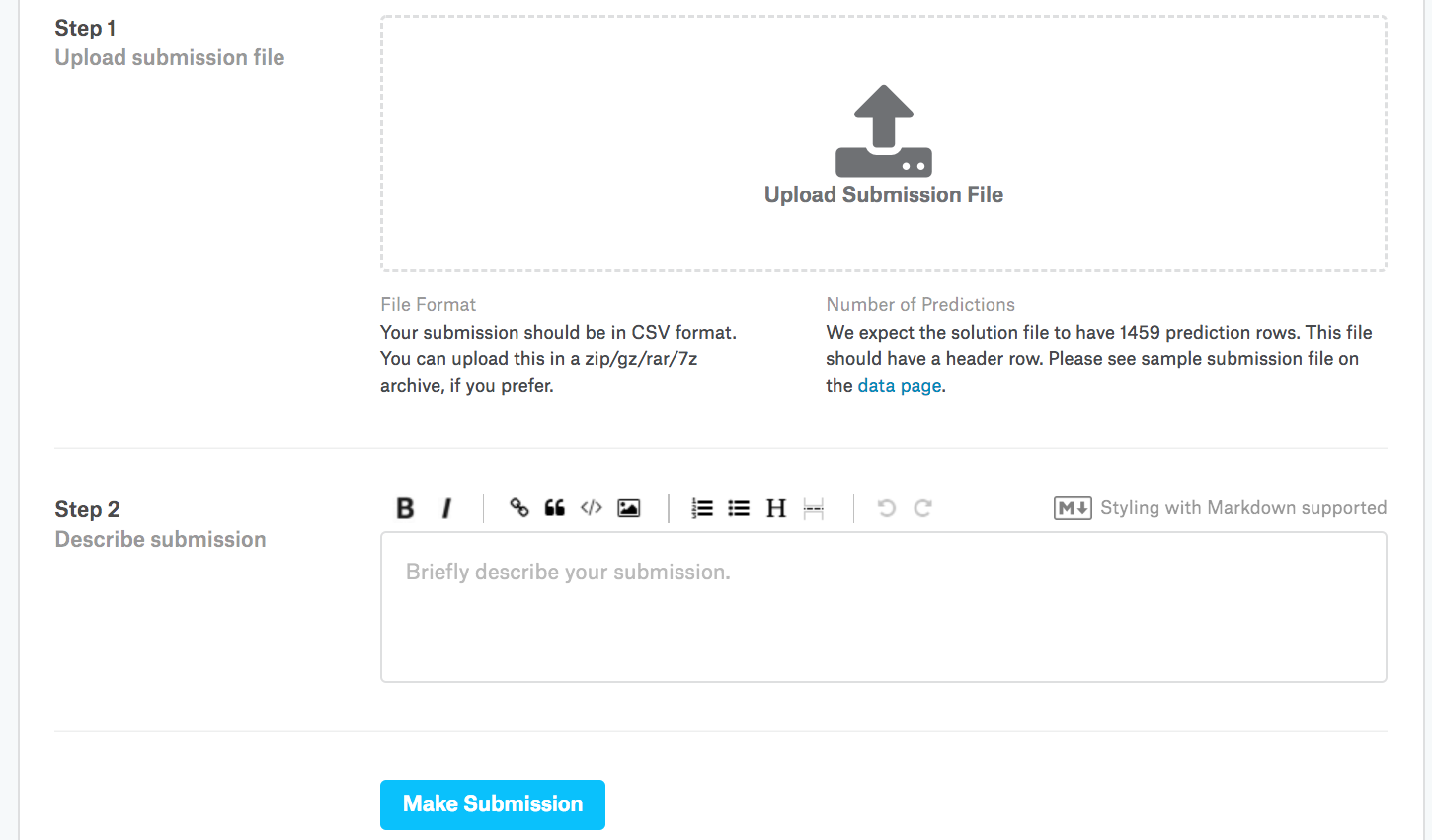
Fig. 5.7.3 Submitting data to Kaggle
5.7.9. Summary and Discussion
Real data often contains a mix of different data types and needs to be preprocessed. Rescaling real-valued data to zero mean and unit variance is a good default. So is replacing missing values with their mean. Furthermore, transforming categorical features into indicator features allows us to treat them like one-hot vectors. When we tend to care more about the relative error than about the absolute error, we can measure the discrepancy in the logarithm of the prediction. To select the model and adjust the hyperparameters, we can use \(K\)-fold cross-validation .
5.7.10. Exercises
Submit your predictions for this section to Kaggle. How good are they?
Is it always a good idea to replace missing values by a mean? Hint: can you construct a situation where the values are not missing at random?
Improve the score by tuning the hyperparameters through \(K\)-fold cross-validation.
Improve the score by improving the model (e.g., layers, weight decay, and dropout).
What happens if we do not standardize the continuous numerical features as we have done in this section?