14.9. Semantic Segmentation and the Dataset¶ Open the notebook in SageMaker Studio Lab
When discussing object detection tasks in Section 14.3–Section 14.8, rectangular bounding boxes are used to label and predict objects in images. This section will discuss the problem of semantic segmentation, which focuses on how to divide an image into regions belonging to different semantic classes. Different from object detection, semantic segmentation recognizes and understands what are in images in pixel level: its labeling and prediction of semantic regions are in pixel level. Fig. 14.9.1 shows the labels of the dog, cat, and background of the image in semantic segmentation. Compared with in object detection, the pixel-level borders labeled in semantic segmentation are obviously more fine-grained.

Fig. 14.9.1 Labels of the dog, cat, and background of the image in semantic segmentation.
14.9.1. Image Segmentation and Instance Segmentation
There are also two important tasks in the field of computer vision that are similar to semantic segmentation, namely image segmentation and instance segmentation. We will briefly distinguish them from semantic segmentation as follows.
Image segmentation divides an image into several constituent regions. The methods for this type of problem usually make use of the correlation between pixels in the image. It does not need label information about image pixels during training, and it cannot guarantee that the segmented regions will have the semantics that we hope to obtain during prediction. Taking the image in Fig. 14.9.1 as input, image segmentation may divide the dog into two regions: one covers the mouth and eyes which are mainly black, and the other covers the rest of the body which is mainly yellow.
Instance segmentation is also called simultaneous detection and segmentation. It studies how to recognize the pixel-level regions of each object instance in an image. Different from semantic segmentation, instance segmentation needs to distinguish not only semantics, but also different object instances. For example, if there are two dogs in the image, instance segmentation needs to distinguish which of the two dogs a pixel belongs to.
14.9.2. The Pascal VOC2012 Semantic Segmentation Dataset
On of the most important semantic segmentation dataset is Pascal VOC2012. In the following, we will take a look at this dataset.
%matplotlib inline
import os
import torch
import torchvision
from d2l import torch as d2l
%matplotlib inline
import os
from mxnet import gluon, image, np, npx
from d2l import mxnet as d2l

npx.set_np()
The tar file of the dataset is about 2 GB, so it may take a while to
download the file. The extracted dataset is located at
../data/VOCdevkit/VOC2012.
#@save
d2l.DATA_HUB['voc2012'] = (d2l.DATA_URL + 'VOCtrainval_11-May-2012.tar',
                           '4e443f8a2eca6b1dac8a6c57641b67dd40621a49')

voc_dir = d2l.download_extract('voc2012', 'VOCdevkit/VOC2012')
Downloading ../data/VOCtrainval_11-May-2012.tar from http://d2l-data.s3-accelerate.amazonaws.com/VOCtrainval_11-May-2012.tar...
After entering the path ../data/VOCdevkit/VOC2012, we can see the
different components of the dataset. The ImageSets/Segmentation path
contains text files that specify training and test samples, while the
JPEGImages and SegmentationClass paths store the input image and
label for each example, respectively. The label here is also in the
image format, with the same size as its labeled input image. Besides,
pixels with the same color in any label image belong to the same
semantic class. The following defines the read_voc_images function
to read all the input images and labels into the memory.
#@save
def read_voc_images(voc_dir, is_train=True):
    """Read all VOC feature and label images."""
    txt_fname = os.path.join(voc_dir, 'ImageSets', 'Segmentation',
                             'train.txt' if is_train else 'val.txt')
    mode = torchvision.io.image.ImageReadMode.RGB
    with open(txt_fname, 'r') as f:
        images = f.read().split()
    features, labels = [], []
    for i, fname in enumerate(images):
        features.append(torchvision.io.read_image(os.path.join(
            voc_dir, 'JPEGImages', f'{fname}.jpg')))
        labels.append(torchvision.io.read_image(os.path.join(
            voc_dir, 'SegmentationClass' ,f'{fname}.png'), mode))
    return features, labels

train_features, train_labels = read_voc_images(voc_dir, True)
#@save
def read_voc_images(voc_dir, is_train=True):
    """Read all VOC feature and label images."""
    txt_fname = os.path.join(voc_dir, 'ImageSets', 'Segmentation',
                             'train.txt' if is_train else 'val.txt')
    with open(txt_fname, 'r') as f:
        images = f.read().split()
    features, labels = [], []
    for i, fname in enumerate(images):
        features.append(image.imread(os.path.join(
            voc_dir, 'JPEGImages', f'{fname}.jpg')))
        labels.append(image.imread(os.path.join(
            voc_dir, 'SegmentationClass', f'{fname}.png')))
    return features, labels

train_features, train_labels = read_voc_images(voc_dir, True)
[22:12:52] ../src/storage/storage.cc:196: Using Pooled (Naive) StorageManager for CPU
We draw the first five input images and their labels. In the label images, white and black represent borders and background, respectively, while the other colors correspond to different classes.
n = 5
imgs = train_features[:n] + train_labels[:n]
imgs = [img.permute(1,2,0) for img in imgs]
d2l.show_images(imgs, 2, n);

n = 5
imgs = train_features[:n] + train_labels[:n]
d2l.show_images(imgs, 2, n);
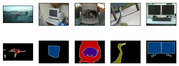
Next, we enumerate the RGB color values and class names for all the labels in this dataset.
#@save
VOC_COLORMAP = [[0, 0, 0], [128, 0, 0], [0, 128, 0], [128, 128, 0],
                [0, 0, 128], [128, 0, 128], [0, 128, 128], [128, 128, 128],
                [64, 0, 0], [192, 0, 0], [64, 128, 0], [192, 128, 0],
                [64, 0, 128], [192, 0, 128], [64, 128, 128], [192, 128, 128],
                [0, 64, 0], [128, 64, 0], [0, 192, 0], [128, 192, 0],
                [0, 64, 128]]

#@save
VOC_CLASSES = ['background', 'aeroplane', 'bicycle', 'bird', 'boat',
               'bottle', 'bus', 'car', 'cat', 'chair', 'cow',
               'diningtable', 'dog', 'horse', 'motorbike', 'person',
               'potted plant', 'sheep', 'sofa', 'train', 'tv/monitor']
#@save
VOC_COLORMAP = [[0, 0, 0], [128, 0, 0], [0, 128, 0], [128, 128, 0],
                [0, 0, 128], [128, 0, 128], [0, 128, 128], [128, 128, 128],
                [64, 0, 0], [192, 0, 0], [64, 128, 0], [192, 128, 0],
                [64, 0, 128], [192, 0, 128], [64, 128, 128], [192, 128, 128],
                [0, 64, 0], [128, 64, 0], [0, 192, 0], [128, 192, 0],
                [0, 64, 128]]

#@save
VOC_CLASSES = ['background', 'aeroplane', 'bicycle', 'bird', 'boat',
               'bottle', 'bus', 'car', 'cat', 'chair', 'cow',
               'diningtable', 'dog', 'horse', 'motorbike', 'person',
               'potted plant', 'sheep', 'sofa', 'train', 'tv/monitor']
With the two constants defined above, we can conveniently find the class
index for each pixel in a label. We define the voc_colormap2label
function to build the mapping from the above RGB color values to class
indices, and the voc_label_indices function to map any RGB values to
their class indices in this Pascal VOC2012 dataset.
#@save
def voc_colormap2label():
    """Build the mapping from RGB to class indices for VOC labels."""
    colormap2label = torch.zeros(256 ** 3, dtype=torch.long)
    for i, colormap in enumerate(VOC_COLORMAP):
        colormap2label[
            (colormap[0] * 256 + colormap[1]) * 256 + colormap[2]] = i
    return colormap2label

#@save
def voc_label_indices(colormap, colormap2label):
    """Map any RGB values in VOC labels to their class indices."""
    colormap = colormap.permute(1, 2, 0).numpy().astype('int32')
    idx = ((colormap[:, :, 0] * 256 + colormap[:, :, 1]) * 256
           + colormap[:, :, 2])
    return colormap2label[idx]
#@save
def voc_colormap2label():
    """Build the mapping from RGB to class indices for VOC labels."""
    colormap2label = np.zeros(256 ** 3)
    for i, colormap in enumerate(VOC_COLORMAP):
        colormap2label[
            (colormap[0] * 256 + colormap[1]) * 256 + colormap[2]] = i
    return colormap2label

#@save
def voc_label_indices(colormap, colormap2label):
    """Map any RGB values in VOC labels to their class indices."""
    colormap = colormap.astype(np.int32)
    idx = ((colormap[:, :, 0] * 256 + colormap[:, :, 1]) * 256
           + colormap[:, :, 2])
    return colormap2label[idx]
For example, in the first example image, the class index for the front part of the airplane is 1, while the background index is 0.
y = voc_label_indices(train_labels[0], voc_colormap2label())
y[105:115, 130:140], VOC_CLASSES[1]
(tensor([[0, 0, 0, 0, 0, 0, 0, 0, 0, 1],
         [0, 0, 0, 0, 0, 0, 0, 1, 1, 1],
         [0, 0, 0, 0, 0, 0, 1, 1, 1, 1],
         [0, 0, 0, 0, 0, 1, 1, 1, 1, 1],
         [0, 0, 0, 0, 0, 1, 1, 1, 1, 1],
         [0, 0, 0, 0, 1, 1, 1, 1, 1, 1],
         [0, 0, 0, 0, 0, 1, 1, 1, 1, 1],
         [0, 0, 0, 0, 0, 1, 1, 1, 1, 1],
         [0, 0, 0, 0, 0, 0, 1, 1, 1, 1],
         [0, 0, 0, 0, 0, 0, 0, 0, 1, 1]]),
 'aeroplane')
y = voc_label_indices(train_labels[0], voc_colormap2label())
y[105:115, 130:140], VOC_CLASSES[1]
(array([[0., 0., 0., 0., 0., 0., 0., 0., 0., 1.],
        [0., 0., 0., 0., 0., 0., 0., 1., 1., 1.],
        [0., 0., 0., 0., 0., 0., 1., 1., 1., 1.],
        [0., 0., 0., 0., 0., 1., 1., 1., 1., 1.],
        [0., 0., 0., 0., 0., 1., 1., 1., 1., 1.],
        [0., 0., 0., 0., 1., 1., 1., 1., 1., 1.],
        [0., 0., 0., 0., 0., 1., 1., 1., 1., 1.],
        [0., 0., 0., 0., 0., 1., 1., 1., 1., 1.],
        [0., 0., 0., 0., 0., 0., 1., 1., 1., 1.],
        [0., 0., 0., 0., 0., 0., 0., 0., 1., 1.]]),
 'aeroplane')
14.9.2.1. Data Preprocessing
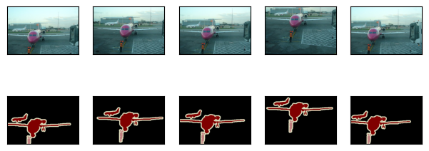
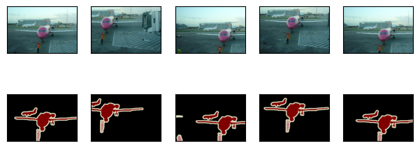
In previous experiments such as in Section 8.1–Section 8.4, images are rescaled to fit the model’s required input shape. However, in semantic segmentation, doing so requires rescaling the predicted pixel classes back to the original shape of the input image. Such rescaling may be inaccurate, especially for segmented regions with different classes. To avoid this issue, we crop the image to a fixed shape instead of rescaling. Specifically, using random cropping from image augmentation, we crop the same area of the input image and the label.
#@save
def voc_rand_crop(feature, label, height, width):
    """Randomly crop both feature and label images."""
    rect = torchvision.transforms.RandomCrop.get_params(
        feature, (height, width))
    feature = torchvision.transforms.functional.crop(feature, *rect)
    label = torchvision.transforms.functional.crop(label, *rect)
    return feature, label

imgs = []
for _ in range(n):
    imgs += voc_rand_crop(train_features[0], train_labels[0], 200, 300)

imgs = [img.permute(1, 2, 0) for img in imgs]
d2l.show_images(imgs[::2] + imgs[1::2], 2, n);
#@save
def voc_rand_crop(feature, label, height, width):
    """Randomly crop both feature and label images."""
    feature, rect = image.random_crop(feature, (width, height))
    label = image.fixed_crop(label, *rect)
    return feature, label

imgs = []
for _ in range(n):
    imgs += voc_rand_crop(train_features[0], train_labels[0], 200, 300)
d2l.show_images(imgs[::2] + imgs[1::2], 2, n);
14.9.2.2. Custom Semantic Segmentation Dataset Class
We define a custom semantic segmentation dataset class VOCSegDataset
by inheriting the Dataset class provided by high-level APIs. By
implementing the __getitem__ function, we can arbitrarily access the
input image indexed as idx in the dataset and the class index of
each pixel in this image. Since some images in the dataset have a
smaller size than the output size of random cropping, these examples are
filtered out by a custom filter function. In addition, we also
define the normalize_image function to standardize the values of the
three RGB channels of input images.
#@save
class VOCSegDataset(torch.utils.data.Dataset):
    """A customized dataset to load the VOC dataset."""

    def __init__(self, is_train, crop_size, voc_dir):
        self.transform = torchvision.transforms.Normalize(
            mean=[0.485, 0.456, 0.406], std=[0.229, 0.224, 0.225])
        self.crop_size = crop_size
        features, labels = read_voc_images(voc_dir, is_train=is_train)
        self.features = [self.normalize_image(feature)
                         for feature in self.filter(features)]
        self.labels = self.filter(labels)
        self.colormap2label = voc_colormap2label()
        print('read ' + str(len(self.features)) + ' examples')

    def normalize_image(self, img):
        return self.transform(img.float() / 255)

    def filter(self, imgs):
        return [img for img in imgs if (
            img.shape[1] >= self.crop_size[0] and
            img.shape[2] >= self.crop_size[1])]

    def __getitem__(self, idx):
        feature, label = voc_rand_crop(self.features[idx], self.labels[idx],
                                       *self.crop_size)
        return (feature, voc_label_indices(label, self.colormap2label))

    def __len__(self):
        return len(self.features)
#@save
class VOCSegDataset(gluon.data.Dataset):
    """A customized dataset to load the VOC dataset."""
    def __init__(self, is_train, crop_size, voc_dir):
        self.rgb_mean = np.array([0.485, 0.456, 0.406])
        self.rgb_std = np.array([0.229, 0.224, 0.225])
        self.crop_size = crop_size
        features, labels = read_voc_images(voc_dir, is_train=is_train)
        self.features = [self.normalize_image(feature)
                         for feature in self.filter(features)]
        self.labels = self.filter(labels)
        self.colormap2label = voc_colormap2label()
        print('read ' + str(len(self.features)) + ' examples')

    def normalize_image(self, img):
        return (img.astype('float32') / 255 - self.rgb_mean) / self.rgb_std

    def filter(self, imgs):
        return [img for img in imgs if (
            img.shape[0] >= self.crop_size[0] and
            img.shape[1] >= self.crop_size[1])]

    def __getitem__(self, idx):
        feature, label = voc_rand_crop(self.features[idx], self.labels[idx],
                                       *self.crop_size)
        return (feature.transpose(2, 0, 1),
                voc_label_indices(label, self.colormap2label))

    def __len__(self):
        return len(self.features)
14.9.2.3. Reading the Dataset
We use the custom VOCSegDataset class to create instances of the
training set and test set, respectively. Suppose that we specify that
the output shape of randomly cropped images is \(320\times 480\).
Below we can view the number of examples that are retained in the
training set and test set.
crop_size = (320, 480)
voc_train = VOCSegDataset(True, crop_size, voc_dir)
voc_test = VOCSegDataset(False, crop_size, voc_dir)
read 1114 examples
read 1078 examples
crop_size = (320, 480)
voc_train = VOCSegDataset(True, crop_size, voc_dir)
voc_test = VOCSegDataset(False, crop_size, voc_dir)
read 1114 examples
read 1078 examples
Setting the batch size to 64, we define the data iterator for the training set. Let’s print the shape of the first minibatch. Different from in image classification or object detection, labels here are three-dimensional tensors.
batch_size = 64
train_iter = torch.utils.data.DataLoader(voc_train, batch_size, shuffle=True,
                                    drop_last=True,
                                    num_workers=d2l.get_dataloader_workers())
for X, Y in train_iter:
    print(X.shape)
    print(Y.shape)
    break
torch.Size([64, 3, 320, 480])
torch.Size([64, 320, 480])
batch_size = 64
train_iter = gluon.data.DataLoader(voc_train, batch_size, shuffle=True,
                                   last_batch='discard',
                                   num_workers=d2l.get_dataloader_workers())
for X, Y in train_iter:
    print(X.shape)
    print(Y.shape)
    break
(64, 3, 320, 480)
(64, 320, 480)
14.9.2.4. Putting It All Together
Finally, we define the following load_data_voc function to download
and read the Pascal VOC2012 semantic segmentation dataset. It returns
data iterators for both the training and test datasets.
#@save
def load_data_voc(batch_size, crop_size):
    """Load the VOC semantic segmentation dataset."""
    voc_dir = d2l.download_extract('voc2012', os.path.join(
        'VOCdevkit', 'VOC2012'))
    num_workers = d2l.get_dataloader_workers()
    train_iter = torch.utils.data.DataLoader(
        VOCSegDataset(True, crop_size, voc_dir), batch_size,
        shuffle=True, drop_last=True, num_workers=num_workers)
    test_iter = torch.utils.data.DataLoader(
        VOCSegDataset(False, crop_size, voc_dir), batch_size,
        drop_last=True, num_workers=num_workers)
    return train_iter, test_iter
#@save
def load_data_voc(batch_size, crop_size):
    """Load the VOC semantic segmentation dataset."""
    voc_dir = d2l.download_extract('voc2012', os.path.join(
        'VOCdevkit', 'VOC2012'))
    num_workers = d2l.get_dataloader_workers()
    train_iter = gluon.data.DataLoader(
        VOCSegDataset(True, crop_size, voc_dir), batch_size,
        shuffle=True, last_batch='discard', num_workers=num_workers)
    test_iter = gluon.data.DataLoader(
        VOCSegDataset(False, crop_size, voc_dir), batch_size,
        last_batch='discard', num_workers=num_workers)
    return train_iter, test_iter
14.9.3. Summary
Semantic segmentation recognizes and understands what are in an image in pixel level by dividing the image into regions belonging to different semantic classes.
One of the most important semantic segmentation dataset is Pascal VOC2012.
In semantic segmentation, since the input image and label correspond one-to-one on the pixel, the input image is randomly cropped to a fixed shape rather than rescaled.
14.9.4. Exercises
How can semantic segmentation be applied in autonomous vehicles and medical image diagnostics? Can you think of other applications?
Recall the descriptions of data augmentation in Section 14.1. Which of the image augmentation methods used in image classification would be infeasible to be applied in semantic segmentation?