9.1. Working with Sequences¶ Open the notebook in SageMaker Studio Lab
Up until now, we have focused on models whose inputs consisted of a single feature vector \(\mathbf{x} \in \mathbb{R}^d\). The main change of perspective when developing models capable of processing sequences is that we now focus on inputs that consist of an ordered list of feature vectors \(\mathbf{x}_1, \dots, \mathbf{x}_T\), where each feature vector \(\mathbf{x}_t\) is indexed by a time step \(t \in \mathbb{Z}^+\) lying in \(\mathbb{R}^d\).
Some datasets consist of a single massive sequence. Consider, for example, the extremely long streams of sensor readings that might be available to climate scientists. In such cases, we might create training datasets by randomly sampling subsequences of some predetermined length. More often, our data arrives as a collection of sequences. Consider the following examples: (i) a collection of documents, each represented as its own sequence of words, and each having its own length \(T_i\); (ii) sequence representation of patient stays in the hospital, where each stay consists of a number of events and the sequence length depends roughly on the length of the stay.
Previously, when dealing with individual inputs, we assumed that they were sampled independently from the same underlying distribution \(P(X)\). While we still assume that entire sequences (e.g., entire documents or patient trajectories) are sampled independently, we cannot assume that the data arriving at each time step are independent of each other. For example, the words that likely to appear later in a document depend heavily on words occurring earlier in the document. The medicine a patient is likely to receive on the 10th day of a hospital visit depends heavily on what transpired in the previous nine days.
This should come as no surprise. If we did not believe that the elements in a sequence were related, we would not have bothered to model them as a sequence in the first place. Consider the usefulness of the auto-fill features that are popular on search tools and modern email clients. They are useful precisely because it is often possible to predict (imperfectly, but better than random guessing) what the likely continuations of a sequence might be, given some initial prefix. For most sequence models, we do not require independence, or even stationarity, of our sequences. Instead, we require only that the sequences themselves are sampled from some fixed underlying distribution over entire sequences.
This flexible approach allows for such phenomena as (i) documents looking significantly different at the beginning than at the end; or (ii) patient status evolving either towards recovery or towards death over the course of a hospital stay; or (iii) customer taste evolving in predictable ways over the course of continued interaction with a recommender system.
We sometimes wish to predict a fixed target \(y\) given sequentially structured input (e.g., sentiment classification based on a movie review). At other times, we wish to predict a sequentially structured target (\(y_1, \ldots, y_T\)) given a fixed input (e.g., image captioning). Still other times, our goal is to predict sequentially structured targets based on sequentially structured inputs (e.g., machine translation or video captioning). Such sequence-to-sequence tasks take two forms: (i) aligned: where the input at each time step aligns with a corresponding target (e.g., part of speech tagging); (ii) unaligned: where the input and target do not necessarily exhibit a step-for-step correspondence (e.g., machine translation).
Before we worry about handling targets of any kind, we can tackle the most straightforward problem: unsupervised density modeling (also called sequence modeling). Here, given a collection of sequences, our goal is to estimate the probability mass function that tells us how likely we are to see any given sequence, i.e., \(p(\mathbf{x}_1, \ldots, \mathbf{x}_T)\).
%matplotlib inline
import torch
from torch import nn
from d2l import torch as d2l
%matplotlib inline
from mxnet import autograd, gluon, init, np, npx
from mxnet.gluon import nn
from d2l import mxnet as d2l

npx.set_np()
%matplotlib inline
import jax
import numpy as np
from jax import numpy as jnp
from d2l import jax as d2l
No GPU/TPU found, falling back to CPU. (Set TF_CPP_MIN_LOG_LEVEL=0 and rerun for more info.)
%matplotlib inline
import tensorflow as tf
from d2l import tensorflow as d2l
9.1.1. Autoregressive Models
Before introducing specialized neural networks designed to handle sequentially structured data, let’s take a look at some actual sequence data and build up some basic intuitions and statistical tools. In particular, we will focus on stock price data from the FTSE 100 index (Fig. 9.1.1). At each time step \(t \in \mathbb{Z}^+\), we observe the price, \(x_t\), of the index at that time.
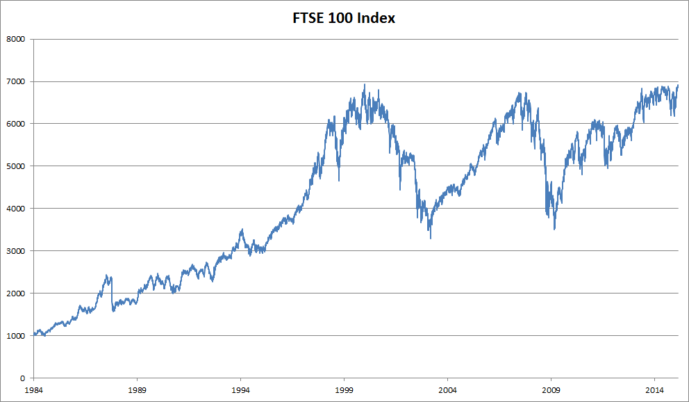
Fig. 9.1.1 FTSE 100 index over about 30 years.
Now suppose that a trader would like to make short-term trades, strategically getting into or out of the index, depending on whether they believe that it will rise or decline in the subsequent time step. Absent any other features (news, financial reporting data, etc.), the only available signal for predicting the subsequent value is the history of prices to date. The trader is thus interested in knowing the probability distribution
over prices that the index might take in the subsequent time step. While estimating the entire distribution over a continuously valued random variable can be difficult, the trader would be happy to focus on a few key statistics of the distribution, particularly the expected value and the variance. One simple strategy for estimating the conditional expectation
would be to apply a linear regression model (recall Section 3.1). Such models that regress the value of a signal on the previous values of that same signal are naturally called autoregressive models. There is just one major problem: the number of inputs, \(x_{t-1}, \ldots, x_1\) varies, depending on \(t\). In other words, the number of inputs increases with the amount of data that we encounter. Thus if we want to treat our historical data as a training set, we are left with the problem that each example has a different number of features. Much of what follows in this chapter will revolve around techniques for overcoming these challenges when engaging in such autoregressive modeling problems where the object of interest is \(P(x_t \mid x_{t-1}, \ldots, x_1)\) or some statistic(s) of this distribution.
A few strategies recur frequently. First of all, we might believe that although long sequences \(x_{t-1}, \ldots, x_1\) are available, it may not be necessary to look back so far in the history when predicting the near future. In this case we might content ourselves to condition on some window of length \(\tau\) and only use \(x_{t-1}, \ldots, x_{t-\tau}\) observations. The immediate benefit is that now the number of arguments is always the same, at least for \(t > \tau\). This allows us to train any linear model or deep network that requires fixed-length vectors as inputs. Second, we might develop models that maintain some summary \(h_t\) of the past observations (see Fig. 9.1.2) and at the same time update \(h_t\) in addition to the prediction \(\hat{x}_t\). This leads to models that estimate not only \(x_t\) with \(\hat{x}_t = P(x_t \mid h_{t})\) but also updates of the form \(h_t = g(h_{t-1}, x_{t-1})\). Since \(h_t\) is never observed, these models are also called latent autoregressive models.

Fig. 9.1.2 A latent autoregressive model.
To construct training data from historical data, one typically creates examples by sampling windows randomly. In general, we do not expect time to stand still. However, we often assume that while the specific values of \(x_t\) might change, the dynamics according to which each subsequent observation is generated given the previous observations do not. Statisticians call dynamics that do not change stationary.
9.1.2. Sequence Models
Sometimes, especially when working with language, we wish to estimate the joint probability of an entire sequence. This is a common task when working with sequences composed of discrete tokens, such as words. Generally, these estimated functions are called sequence models and for natural language data, they are called language models. The field of sequence modeling has been driven so much by natural language processing, that we often describe sequence models as “language models”, even when dealing with non-language data. Language models prove useful for all sorts of reasons. Sometimes we want to evaluate the likelihood of sentences. For example, we might wish to compare the naturalness of two candidate outputs generated by a machine translation system or by a speech recognition system. But language modeling gives us not only the capacity to evaluate likelihood, but the ability to sample sequences, and even to optimize for the most likely sequences.
While language modeling might not, at first glance, look like an autoregressive problem, we can reduce language modeling to autoregressive prediction by decomposing the joint density of a sequence \(p(x_1, \ldots, x_T)\) into the product of conditional densities in a left-to-right fashion by applying the chain rule of probability:
Note that if we are working with discrete signals such as words, then the autoregressive model must be a probabilistic classifier, outputting a full probability distribution over the vocabulary for whatever word will come next, given the leftwards context.
9.1.2.1. Markov Models
Now suppose that we wish to employ the strategy mentioned above, where we condition only on the \(\tau\) previous time steps, i.e., \(x_{t-1}, \ldots, x_{t-\tau}\), rather than the entire sequence history \(x_{t-1}, \ldots, x_1\). Whenever we can throw away the history beyond the previous \(\tau\) steps without any loss in predictive power, we say that the sequence satisfies a Markov condition, i.e., that the future is conditionally independent of the past, given the recent history. When \(\tau = 1\), we say that the data is characterized by a first-order Markov model, and when \(\tau = k\), we say that the data is characterized by a \(k^{\textrm{th}}\)-order Markov model. For when the first-order Markov condition holds (\(\tau = 1\)) the factorization of our joint probability becomes a product of probabilities of each word given the previous word:
We often find it useful to work with models that proceed as though a Markov condition were satisfied, even when we know that this is only approximately true. With real text documents we continue to gain information as we include more and more leftwards context. But these gains diminish rapidly. Thus, sometimes we compromise, obviating computational and statistical difficulties by training models whose validity depends on a \(k^{\textrm{th}}\)-order Markov condition. Even today’s massive RNN- and Transformer-based language models seldom incorporate more than thousands of words of context.
With discrete data, a true Markov model simply counts the number of times that each word has occurred in each context, producing the relative frequency estimate of \(P(x_t \mid x_{t-1})\). Whenever the data assumes only discrete values (as in language), the most likely sequence of words can be computed efficiently using dynamic programming.
9.1.2.2. The Order of Decoding
You may be wondering why we represented the factorization of a text sequence \(P(x_1, \ldots, x_T)\) as a left-to-right chain of conditional probabilities. Why not right-to-left or some other, seemingly random order? In principle, there is nothing wrong with unfolding \(P(x_1, \ldots, x_T)\) in reverse order. The result is a valid factorization:
However, there are many reasons why factorizing text in the same direction in which we read it (left-to-right for most languages, but right-to-left for Arabic and Hebrew) is preferred for the task of language modeling. First, this is just a more natural direction for us to think about. After all we all read text every day, and this process is guided by our ability to anticipate which words and phrases are likely to come next. Just think of how many times you have completed someone else’s sentence. Thus, even if we had no other reason to prefer such in-order decodings, they would be useful if only because we have better intuitions for what should be likely when predicting in this order.
Second, by factorizing in order, we can assign probabilities to arbitrarily long sequences using the same language model. To convert a probability over steps \(1\) through \(t\) into one that extends to word \(t+1\) we simply multiply by the conditional probability of the additional token given the previous ones: \(P(x_{t+1}, \ldots, x_1) = P(x_{t}, \ldots, x_1) \cdot P(x_{t+1} \mid x_{t}, \ldots, x_1)\).
Third, we have stronger predictive models for predicting adjacent words than words at arbitrary other locations. While all orders of factorization are valid, they do not necessarily all represent equally easy predictive modeling problems. This is true not only for language, but for other kinds of data as well, e.g., when the data is causally structured. For example, we believe that future events cannot influence the past. Hence, if we change \(x_t\), we may be able to influence what happens for \(x_{t+1}\) going forward but not the converse. That is, if we change \(x_t\), the distribution over past events will not change. In some contexts, this makes it easier to predict \(P(x_{t+1} \mid x_t)\) than to predict \(P(x_t \mid x_{t+1})\). For instance, in some cases, we can find \(x_{t+1} = f(x_t) + \epsilon\) for some additive noise \(\epsilon\), whereas the converse is not true (Hoyer et al., 2009). This is great news, since it is typically the forward direction that we are interested in estimating. The book by Peters et al. (2017) contains more on this topic. We barely scratch the surface of it.
9.1.3. Training
Before we focus our attention on text data, let’s first try this out with some continuous-valued synthetic data.
Here, our 1000 synthetic data will follow the trigonometric sin
function, applied to 0.01 times the time step. To make the problem a
little more interesting, we corrupt each sample with additive noise.
From this sequence we extract training examples, each consisting of
features and a label.
class Data(d2l.DataModule):
    def __init__(self, batch_size=16, T=1000, num_train=600, tau=4):
        self.save_hyperparameters()
        self.time = torch.arange(1, T + 1, dtype=torch.float32)
        self.x = torch.sin(0.01 * self.time) + torch.randn(T) * 0.2

data = Data()
d2l.plot(data.time, data.x, 'time', 'x', xlim=[1, 1000], figsize=(6, 3))

class Data(d2l.DataModule):
    def __init__(self, batch_size=16, T=1000, num_train=600, tau=4):
        self.save_hyperparameters()
        self.time = np.arange(1, T + 1, dtype=np.float32)
        self.x = np.sin(0.01 * self.time) + np.random.randn(T) * 0.2

data = Data()
d2l.plot(data.time, data.x, 'time', 'x', xlim=[1, 1000], figsize=(6, 3))
[22:06:39] ../src/storage/storage.cc:196: Using Pooled (Naive) StorageManager for CPU

class Data(d2l.DataModule):
    def __init__(self, batch_size=16, T=1000, num_train=600, tau=4):
        self.save_hyperparameters()
        self.time = jnp.arange(1, T + 1, dtype=jnp.float32)
        key = d2l.get_key()
        self.x = jnp.sin(0.01 * self.time) + jax.random.normal(key,
                                                               [T]) * 0.2

data = Data()
d2l.plot(data.time, data.x, 'time', 'x', xlim=[1, 1000], figsize=(6, 3))

class Data(d2l.DataModule):
    def __init__(self, batch_size=16, T=1000, num_train=600, tau=4):
        self.save_hyperparameters()
        self.time = tf.range(1, T + 1, dtype=tf.float32)
        self.x = tf.sin(0.01 * self.time) + tf.random.normal([T]) * 0.2

data = Data()
d2l.plot(data.time, data.x, 'time', 'x', xlim=[1, 1000], figsize=(6, 3))

To begin, we try a model that acts as if the data satisfied a \(\tau^{\textrm{th}}\)-order Markov condition, and thus predicts \(x_t\) using only the past \(\tau\) observations. Thus for each time step we have an example with label \(y = x_t\) and features \(\mathbf{x}_t = [x_{t-\tau}, \ldots, x_{t-1}]\). The astute reader might have noticed that this results in \(1000-\tau\) examples, since we lack sufficient history for \(y_1, \ldots, y_\tau\). While we could pad the first \(\tau\) sequences with zeros, to keep things simple, we drop them for now. The resulting dataset contains \(T - \tau\) examples, where each input to the model has sequence length \(\tau\). We create a data iterator on the first 600 examples, covering a period of the sin function.
@d2l.add_to_class(Data)
def get_dataloader(self, train):
    features = [self.x[i : self.T-self.tau+i] for i in range(self.tau)]
    self.features = torch.stack(features, 1)
    self.labels = self.x[self.tau:].reshape((-1, 1))
    i = slice(0, self.num_train) if train else slice(self.num_train, None)
    return self.get_tensorloader([self.features, self.labels], train, i)
@d2l.add_to_class(Data)
def get_dataloader(self, train):
    features = [self.x[i : self.T-self.tau+i] for i in range(self.tau)]
    self.features = np.stack(features, 1)
    self.labels = self.x[self.tau:].reshape((-1, 1))
    i = slice(0, self.num_train) if train else slice(self.num_train, None)
    return self.get_tensorloader([self.features, self.labels], train, i)
@d2l.add_to_class(Data)
def get_dataloader(self, train):
    features = [self.x[i : self.T-self.tau+i] for i in range(self.tau)]
    self.features = jnp.stack(features, 1)
    self.labels = self.x[self.tau:].reshape((-1, 1))
    i = slice(0, self.num_train) if train else slice(self.num_train, None)
    return self.get_tensorloader([self.features, self.labels], train, i)
@d2l.add_to_class(Data)
def get_dataloader(self, train):
    features = [self.x[i : self.T-self.tau+i] for i in range(self.tau)]
    self.features = tf.stack(features, 1)
    self.labels = tf.reshape(self.x[self.tau:], (-1, 1))
    i = slice(0, self.num_train) if train else slice(self.num_train, None)
    return self.get_tensorloader([self.features, self.labels], train, i)
In this example our model will be a standard linear regression.
model = d2l.LinearRegression(lr=0.01)
trainer = d2l.Trainer(max_epochs=5)
trainer.fit(model, data)

model = d2l.LinearRegression(lr=0.01)
trainer = d2l.Trainer(max_epochs=5)
trainer.fit(model, data)

model = d2l.LinearRegression(lr=0.01)
trainer = d2l.Trainer(max_epochs=5)
trainer.fit(model, data)

model = d2l.LinearRegression(lr=0.01)
trainer = d2l.Trainer(max_epochs=5)
trainer.fit(model, data)

9.1.4. Prediction
To evaluate our model, we first check how well it performs at one-step-ahead prediction.
onestep_preds = model(data.features).detach().numpy()
d2l.plot(data.time[data.tau:], [data.labels, onestep_preds], 'time', 'x',
         legend=['labels', '1-step preds'], figsize=(6, 3))

onestep_preds = model(data.features).asnumpy()
d2l.plot(data.time[data.tau:], [data.labels, onestep_preds], 'time', 'x',
         legend=['labels', '1-step preds'], figsize=(6, 3))

onestep_preds = model.apply({'params': trainer.state.params}, data.features)
d2l.plot(data.time[data.tau:], [data.labels, onestep_preds], 'time', 'x',
         legend=['labels', '1-step preds'], figsize=(6, 3))

onestep_preds = model(data.features).numpy()
d2l.plot(data.time[data.tau:], [data.labels, onestep_preds], 'time', 'x',
         legend=['labels', '1-step preds'], figsize=(6, 3))

These predictions look good, even near the end at \(t=1000\).
But what if we only observed sequence data up until time step 604
(n_train + tau) and wished to make predictions several steps into
the future? Unfortunately, we cannot directly compute the one-step-ahead
prediction for time step 609, because we do not know the corresponding
inputs, having seen only up to \(x_{604}\). We can address this
problem by plugging in our earlier predictions as inputs to our model
for making subsequent predictions, projecting forward, one step at a
time, until reaching the desired time step:
Generally, for an observed sequence \(x_1, \ldots, x_t\), its predicted output \(\hat{x}_{t+k}\) at time step \(t+k\) is called the \(k\)-step-ahead prediction. Since we have observed up to \(x_{604}\), its \(k\)-step-ahead prediction is \(\hat{x}_{604+k}\). In other words, we will have to keep on using our own predictions to make multistep-ahead predictions. Let’s see how well this goes.
multistep_preds = torch.zeros(data.T)
multistep_preds[:] = data.x
for i in range(data.num_train + data.tau, data.T):
    multistep_preds[i] = model(
        multistep_preds[i - data.tau:i].reshape((1, -1)))
multistep_preds = multistep_preds.detach().numpy()

d2l.plot([data.time[data.tau:], data.time[data.num_train+data.tau:]],
         [onestep_preds, multistep_preds[data.num_train+data.tau:]], 'time',
         'x', legend=['1-step preds', 'multistep preds'], figsize=(6, 3))

multistep_preds = np.zeros(data.T)
multistep_preds[:] = data.x
for i in range(data.num_train + data.tau, data.T):
    multistep_preds[i] = model(
        multistep_preds[i - data.tau:i].reshape((1, -1)))
multistep_preds = multistep_preds.asnumpy()

d2l.plot([data.time[data.tau:], data.time[data.num_train+data.tau:]],
         [onestep_preds, multistep_preds[data.num_train+data.tau:]], 'time',
         'x', legend=['1-step preds', 'multistep preds'], figsize=(6, 3))

multistep_preds = jnp.zeros(data.T)
multistep_preds = multistep_preds.at[:].set(data.x)
for i in range(data.num_train + data.tau, data.T):
    pred = model.apply({'params': trainer.state.params},
                       multistep_preds[i - data.tau:i].reshape((1, -1)))
    multistep_preds = multistep_preds.at[i].set(pred.item())

d2l.plot([data.time[data.tau:], data.time[data.num_train+data.tau:]],
         [onestep_preds, multistep_preds[data.num_train+data.tau:]], 'time',
         'x', legend=['1-step preds', 'multistep preds'], figsize=(6, 3))

multistep_preds = tf.Variable(tf.zeros(data.T))
multistep_preds[:].assign(data.x)
for i in range(data.num_train + data.tau, data.T):
    multistep_preds[i].assign(tf.reshape(model(
        tf.reshape(multistep_preds[i-data.tau : i], (1, -1))), ()))

d2l.plot([data.time[data.tau:], data.time[data.num_train+data.tau:]],
         [onestep_preds, multistep_preds[data.num_train+data.tau:]], 'time',
         'x', legend=['1-step preds', 'multistep preds'], figsize=(6, 3))

Unfortunately, in this case we fail spectacularly. The predictions decay to a constant pretty quickly after a few steps. Why did the algorithm perform so much worse when predicting further into the future? Ultimately, this is down to the fact that errors build up. Let’s say that after step 1 we have some error \(\epsilon_1 = \bar\epsilon\). Now the input for step 2 is perturbed by \(\epsilon_1\), hence we suffer some error in the order of \(\epsilon_2 = \bar\epsilon + c \epsilon_1\) for some constant \(c\), and so on. The predictions can diverge rapidly from the true observations. You may already be familiar with this common phenomenon. For instance, weather forecasts for the next 24 hours tend to be pretty accurate but beyond that, accuracy declines rapidly. We will discuss methods for improving this throughout this chapter and beyond.
Let’s take a closer look at the difficulties in \(k\)-step-ahead predictions by computing predictions on the entire sequence for \(k = 1, 4, 16, 64\).
def k_step_pred(k):
    features = []
    for i in range(data.tau):
        features.append(data.x[i : i+data.T-data.tau-k+1])
    # The (i+tau)-th element stores the (i+1)-step-ahead predictions
    for i in range(k):
        preds = model(torch.stack(features[i : i+data.tau], 1))
        features.append(preds.reshape(-1))
    return features[data.tau:]

steps = (1, 4, 16, 64)
preds = k_step_pred(steps[-1])
d2l.plot(data.time[data.tau+steps[-1]-1:],
         [preds[k - 1].detach().numpy() for k in steps], 'time', 'x',
         legend=[f'{k}-step preds' for k in steps], figsize=(6, 3))

def k_step_pred(k):
    features = []
    for i in range(data.tau):
        features.append(data.x[i : i+data.T-data.tau-k+1])
    # The (i+tau)-th element stores the (i+1)-step-ahead predictions
    for i in range(k):
        preds = model(np.stack(features[i : i+data.tau], 1))
        features.append(preds.reshape(-1))
    return features[data.tau:]

steps = (1, 4, 16, 64)
preds = k_step_pred(steps[-1])
d2l.plot(data.time[data.tau+steps[-1]-1:],
         [preds[k - 1].asnumpy() for k in steps], 'time', 'x',
         legend=[f'{k}-step preds' for k in steps], figsize=(6, 3))

def k_step_pred(k):
    features = []
    for i in range(data.tau):
        features.append(data.x[i : i+data.T-data.tau-k+1])
    # The (i+tau)-th element stores the (i+1)-step-ahead predictions
    for i in range(k):
        preds = model.apply({'params': trainer.state.params},
                            jnp.stack(features[i : i+data.tau], 1))
        features.append(preds.reshape(-1))
    return features[data.tau:]

steps = (1, 4, 16, 64)
preds = k_step_pred(steps[-1])
d2l.plot(data.time[data.tau+steps[-1]-1:],
         [np.asarray(preds[k-1]) for k in steps], 'time', 'x',
         legend=[f'{k}-step preds' for k in steps], figsize=(6, 3))

def k_step_pred(k):
    features = []
    for i in range(data.tau):
        features.append(data.x[i : i+data.T-data.tau-k+1])
    # The (i+tau)-th element stores the (i+1)-step-ahead predictions
    for i in range(k):
        preds = model(tf.stack(features[i : i+data.tau], 1))
        features.append(tf.reshape(preds, -1))
    return features[data.tau:]

steps = (1, 4, 16, 64)
preds = k_step_pred(steps[-1])
d2l.plot(data.time[data.tau+steps[-1]-1:],
         [preds[k - 1].numpy() for k in steps], 'time', 'x',
         legend=[f'{k}-step preds' for k in steps], figsize=(6, 3))

This clearly illustrates how the quality of the prediction changes as we try to predict further into the future. While the 4-step-ahead predictions still look good, anything beyond that is almost useless.
9.1.5. Summary
There is quite a difference in difficulty between interpolation and extrapolation. Consequently, if you have a sequence, always respect the temporal order of the data when training, i.e., never train on future data. Given this kind of data, sequence models require specialized statistical tools for estimation. Two popular choices are autoregressive models and latent-variable autoregressive models. For causal models (e.g., time going forward), estimating the forward direction is typically a lot easier than the reverse direction. For an observed sequence up to time step \(t\), its predicted output at time step \(t+k\) is the \(k\)-step-ahead prediction. As we predict further in time by increasing \(k\), the errors accumulate and the quality of the prediction degrades, often dramatically.
9.1.6. Exercises
Improve the model in the experiment of this section.
Incorporate more than the past four observations? How many do you really need?
How many past observations would you need if there was no noise? Hint: you can write \(\sin\) and \(\cos\) as a differential equation.
Can you incorporate older observations while keeping the total number of features constant? Does this improve accuracy? Why?
Change the neural network architecture and evaluate the performance. You may train the new model with more epochs. What do you observe?
An investor wants to find a good security to buy. They look at past returns to decide which one is likely to do well. What could possibly go wrong with this strategy?
Does causality also apply to text? To which extent?
Give an example for when a latent autoregressive model might be needed to capture the dynamic of the data.